
By: Fakharyar Khan
Note: Some of the Physics symbols do not translate well into website format. To read a version of this article with the proper formatting please click here.
Diving into Pendulums
From tether ball to the high school lab room and even “spiritual” pendulums, pendulums have always been a great source of entertainment. But they also have been the subject of interest for many mathematicians and physicists.
The Basic Pendulum
A pendulum is a mass suspended from a fixed point that swings back and forth about that point. The gravitational force is broken into a centripetal and tangential force. Using a little bit of trigonometry, we find that the tangential force is F = - mgsin. The negative sign is due to the fact that the acceleration of the pendulum acts in the opposite direction of increasing angle and this is what gives the pendulum its oscillating motion. From this, we have that a = -gsin📷
We also know that the arc length is given by s = L and by taking the derivative on both sides of the equation, we get v = Lddt. We can then take the derivative once again to get a = Ld2dt2. This means that Ld2dt2 =-gsin and so d2dt2 + gLsin = 0. This is called a differential equation and it describes the behavior of functions. Solving this equation will give us as a function of time and allows us to describe the pendulum’s motion easily.
For small angles, we can say that sinwhich then gives us d2dt2 + gL = 0. This is the differential equation of the simple harmonic oscillator and assuming that the initial conditions areddt= 0and (0) = 0, one solution is (t) =0cos(glt) .(a derivation of the solution to the differential equation of the simple harmonic oscillator is in the Elastic Pendulum section) We can now describe the position, velocity, and acceleration of the pendulum at any given time.
The Elastic Pendulum

What if, the string of the pendulum was elastic? There are two types of forces in this system; the restoring force of the string and the gravitational force exerted by the mass.
In the above section, it was more convenient to track the pendulum’s motion by its angle because it followed a circular path. But in the elastic pendulum, since the restoring force relies and is applied on the length of the string, it can be broken up into its vector components.
Imagine a cartesian coordinate system where the fixed point of our pendulum is located at the origin. If we let r(t) represent the position vector of the pendulum as a function of time then L(t)is the magnitude of r(t) at time t. The force of the string will be Fstring=-kr(t)which then can be broken into its vector components to get Fstring=-kx(t)i-ky(t)j. The gravitational force is applied along the y axis so it’s just Fg=-mgj. We can then add both forces to get together to get the resultant and divide by the mass of the pendulum on both sides to obtain the total acceleration: a = -kmx(t)i-g*ky(t)j. We can then split them up into their vector components to get: x" =-kmx(t) and y" =-g*ky(t).
For both equations, the acceleration is just the position function multiplied by some constant which means that x(t) = Aeikmt and y(t) = Beigktwhere A and B are constants of integration. By Euler’s Formula, one solution for x(t) is cos(kmt)+isin(kmt)where A = 1 another is cos(kmt)-isin(kmt) . If we make i the constant of integration, then we get icos(kmt)-sin(kmt) and icos(kmt)+sin(kmt). Because these two functions satisfy the differential equation, any linear combination of the two functions satisfies it as well since derivatives are linear operators meaning ((f(x) + g(x))' = f(x)' + g(x)'and [cf(x)]'=c(f(x))'. Therefore, we can add the first two solutions to get x(t) =cos(kmt) and add the second two equations to get x(t) =sin(kmt) . A linear combination of these two solutions will then give us x(t) = Acos(kmt)+Bsin(kmt) . We can use this same idea to solve the differential equation for the normal pendulum. Similarly,y(t) = Dcos(gkt)+Esin(gkt). We now have a set of parametric equations to model the motion! 📷
The graph to the left shows the motion of the pendulum with k = 500 N and m = 0.23 kg. If you click on the link here https://www.desmos.com/calculator/aw68zx9wj9 , you can play around with the spring constant and mass. One really cool thing is that when the mass is between 0 and 1 kg, the graph of the pendulum’s motion changes wildly and after that, the graph changes almost periodically. On average, the graph became like this every 2.6 seconds.
Double Pendulums

A double pendulum is where one pendulum is attached to another. The double pendulum is a classic example of chaotic motion because if the initial conditions, the initial velocity, position, and acceleration, are just slightly different, it would follow a completely different trajectory as can be seen in the simulation of three double pendulums to the right. Our goal is to find and solve a differential equation that describes the pendulum’s motion.
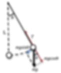
Using the figure below as our free body diagram, the position of the first pendulum is at (x1, y1)= (L1sin1,−L1cos θ1) and the second is at (x2, y2)=(L1sin1+L2sin2,-L1cos1-L2cos2) .
The direction of the horizontal component of the tension in the first string is opposite that of the direction of the horizontal component of the tension in the second string. This is because when the first pendulum moves clockwise, the second pendulum will experience an opposite force that will move it counterclockwise. Therefore, Fnet,x1=m1 x1''=−T1 sin θ1 + T2 sin θ2, where x''represents the second time derivative of x, is the horizontal net force in the first pendulum. The vertical net force has the gravitational force of the first mass and the vertical components of the tension in both strings. Fnet,y1=m1 y1'' = T1 cos θ1 − T2 cos θ2 − m1 g.📷
The lower pendulum is only influenced by its string’s tension and the gravitational force of its mass. Thus, Fnet,x2= m2 x2'' = -T2sin θ2 and Fnet,y2=m2 y2'' = T2 cos θ2 − m2 g.
We now want to eliminate all terms that contain tension so that we can write θ1"and θ2"purely in terms of angular velocity and angular displacement. We know that -m2 x2'' = T2sin θ2 and so we can substitute this back into the equation for horizontal net force of the first pendulum to get m1 x1''=−T1 sin θ1 -m2 x2'' . We then have that m2 y2''= T2 cos θ2 -m2 gwhich we can substitute vertical net force in the second pendulum in the equation for the vertical net force in first pendulum to get m1 y1'' = T1 cos θ1 − m2 y2'' − m2 g − m1 g. (Note: The substitution of m2 y2'' introduced the term m2 ginto the equation). If we isolate the terms in the two equations we have that contain tension we get, T1 cos θ1=m1 y1'' + m2 y2'' + m2 g +m1g and T1 sin θ1= -m1 y1'' -m2 y2''.
If we multiply the first equation by sin θ1and the second by cos θ1, we get equivalent expressions for T1 cos θ1sin θ1. We now have an equation that relates θ1 to its derivatives.
1=sin θ1 (m1 y1'' + m2 y2'' + m2 g + m1 g) = −cos θ1 (m1 x1'' + m2x2'')
We now aim to the same with θ2. Luckily, the dynamics of the second pendulum is only reliant on the tension in the second string so we can solve the horizontal and vertical component equations for their tension terms and then multiply them by either sin2or cos2 so that they are equal to each other. This gets us the second equation:2=sin θ2(m2 y2'' + m2 g)= −cos θ2 (m2 x2'').
Using a computer program, we can now isolate these equations for θ1"and θ2" to finally get the differential equations:
θ1'' = −g (2 m1 + m2) sin θ1 − m2 g sin(θ1 − 2 θ2) − 2 sin(θ1 − θ2) m2 (θ2'2 L2 + θ1'2 L1 cos(θ1 − θ2))L1 (2 m1 + m2 − m2 cos(2 θ1 − 2 θ2))
θ2'' = 2 sin(θ1 − θ2) (θ1'2 L1 (m1 + m2) + g(m1 + m2) cos θ1 + θ2'2 L2 m2 cos(θ1 − θ2))L2 (2 m1 + m2 − m2 cos(2 θ1 − 2 θ2))
It is impossible to find a solution in terms of elementary functions (functions that are integrable) to this set of differential equations would be so instead we can use techniques like Euler’s method to approximate the motion to any desired accuracy.
N-Pendulums Taken to Infinity
One way we could continue the topic of pendulums is by describing a general system of n pendulums. This problem is also called the “Hanging Chain” and it was solved in the 18th century by the mathematicians Daniel Bernoulli and Leonard Euler. For small oscillations, they found that for the ith pendulum, it’s motion can be approximated purely horizontally as such:
xi''=g[(n-i)(xi+1-xiai+1-xi-xi-1ai)-(xi-xi-1ai), where ai is the length of the ith string attached to the ith pendulum. Ryan Rubenzahl is an undergraduate at the University of Rochester who gives a really nice derivation of this equation using Newtonian Dynamics in his term paper here.
If we now take n to infinity, the rope is continuous, in the sense that it is of constant density. The motion of the ith pendulum then describes the motion of the rope at that location. But since the rope is continuous, the motion of the ith pendulum must describe the general movement of the rope. Therefore, nxi''=2x(y,t)t2. Assuming that the length of each string, aiare equal, we can write the limit as ng[(n-i)*a*1a(xi+1-xia-xi-xi-1a) -(xi-xi-1a). We now can evaluate the limit by breaking it into parts. Since n*a represents the full length of the rope and i * a represents the vertical position of the pendulum, n(n-i)*a =(l-y) . xi-xi-1arepresents the change in x over the change in y since a represents the vertical length between each pendulum. As n approaches infinity, a will approach zero so really n(xi-xi-1a)is just x(y,t)y, the partial derivative of x with respect to y. The last term is: 1a(xi+1-xia-xi-xi-1a)which is really just the change of the change in x with respect to y so taken to infinity we have: n1a(xi+1-xia-xi-xi-1a)=2x(y,t)y2. Taking it all together, we have nxi''=2xt2=g[(l-y)2xy2-xy]. This equation is known as the wave equation and comes up frequently in many areas of classical physics. The solution to the wave equation is difficult to derive but it is solvable, just… not recommended.
Conclusion
Pendulum systems are really fun to analyze. And we have barely scratched the surface of pendulum systems. The pendulum cart, inverted pendulum (and its stabilization is a very popular topic in control theory), the torsion pendulum, and the coupled pendulum are a couple of them.
Sources
(n.d.). Applications of vibration models. Retrieved from http://hplgit.github.io/fdm-book/doc/pub/book/html/._fdm-book005.html
Double Pendulum. Retrieved from https://www.myphysicslab.com/pendulum/double-pendulum-en.html
https://www.webassign.net/question_assets/ncsucalcphysmechl3/lab_7_1/manual.html
(2019, March 6). Chaos and the Double Pendulum. Retrieved from https://gereshes.com/2018/11/19/chaos-and-the-double-pendulum/
Assencio, D. (n.d.). Retrieved from https://diego.assencio.com/?index=1500c66ae7ab27bb0106467c68feebc6